Getting live tide and swell data with tesseract and rvest

The Department of Transport publishes live tide and swell data, which can be scraped using just a few lines of R code.

Sea and swell

The Western Australia Department of Transport has a wave buoy recording swell data off Cottesloe. The historical data is an incredibly useful resource, but what if you wanted to use the conditions right now? There is a DOT website that provides the current readings, but only in image format. Here is one from when I wrote this post.

Cottesloe sea and swell product for 22nd Jan 2022

It is possible to read the sea and swell height directly from the image using the tesseract package. This performs optical character recognition, extracting text from any image. The magick package can be used to clean up the image, before piping it into the ocr() function. This returns a character string:

library(tidyverse)
library(tesseract)
library(magick)

url <- "https://www.transport.wa.gov.au/imarine/coastaldata/tidesandwaves/live_gfx/DWM_POLD.gif"
input <- image_read(url)

text <- input %>%
  image_convert(type = 'Grayscale') %>%
  image_crop("140x76+0+20") %>% 
  image_write(format = 'png', density = '300x300') %>%
  tesseract::ocr() 

text

[1] "SEA 0.37m\nSWELL 0.37m\n"

From there, some trivial data cleaning using the tidyverse can turn this string into a tibble (rectangular data frame).

waves <- tibble(
  m = str_split(text, pattern = "\\n") %>% unlist()) %>%
  separate(m, into = c("wave", "m"), sep = " ") %>% 
  drop_na() %>% 
  mutate(wave = str_to_lower(wave),
         m = parse_number(m))

waves

# A tibble: 2 × 2
  wave      m
  <chr> <dbl>
1 sea    0.37
2 swell  0.37

Tides

The tide data for Fishing Boat Harbour in Fremantle is presented on a webpage, which can be scraped using rvest.

Screenshot of tide webpage on 22nd Jan 2022

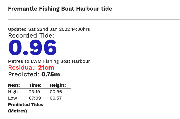
First you read the webpage in, and select all the span elements. The current tide is the only span on the page in large blue font, so you can select it by that attribute, and convert it to a number.

library(rvest)
url <- "https://www.transport.wa.gov.au/imarine/fremantle-fishing-boat-harbour-tide.asp"

nodes <- read_html(url) %>%
  html_nodes("span")

font <-  "font-size:72px;font-weight:bold;color:#0000AA"
index <- which(html_attr(nodes, 'style') == font)

tide = nodes[index] %>% html_text() %>% as.double()
tide

[1] 0.96

Combining and logging

You can add the tide observations to swell with the add_row function, then reshape it to a more appropriate format and add the current time.

waves <- waves %>% add_row(wave = 'tide', m = tide)

latest <- waves %>%
  pivot_wider(names_from = wave, values_from = m) %>% 
  mutate(t = Sys.time())

latest

# A tibble: 1 × 4
    sea swell  tide t                  
  <dbl> <dbl> <dbl> <dttm>             
1  0.37  0.37  0.96 2022-01-22 14:46:43

The final line appends this to an existing csv. You should run it once first with append=FALSE to create the header row.

write_csv(latest, 'waves.csv', append = TRUE)

With the complete code in a single file, it can be run every 20 minutes to log the data, using just a while loop and sys.sleep.

while (TRUE) {
  source('')
  print('logged')
  print(latest)
  Sys.sleep(20*60)
}

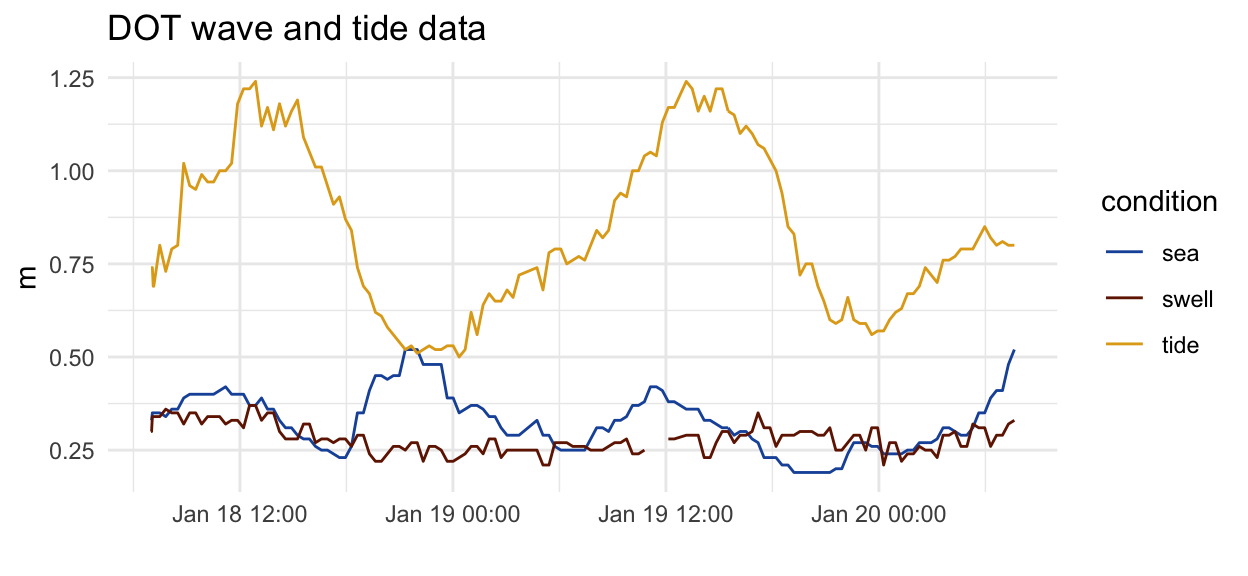
Here is the result of running this over a couple of days.

logged <- read_csv('waves.csv') %>%
  pivot_longer(cols = sea:tide,
               names_to = 'condition',
               values_to = 'm')

ggplot(logged, aes(t, m)) +
  geom_line(aes(colour = condition)) + 
  labs(x = "", title = 'DOT wave and tide data') +
  theme_minimal() +
  scale_colour_manual(
    values = c(
      "sea" = '#1B54A8',
      "swell" = '#701C00',
      'tide' = "#E1A81C")
    )

complete code

library(tidyverse)
library(tesseract)
library(magick)
library(rvest)

input <- image_read("https://www.transport.wa.gov.au/imarine/coastaldata/tidesandwaves/live_gfx/DWM_POLD.gif")

text <- input %>%
  image_convert(type = 'Grayscale') %>%
  image_crop("140x76+0+20") %>% 
  image_write(format = 'png', density = '300x300') %>%
  tesseract::ocr() 

waves <- tibble(
  m = str_split(text, pattern = "\\n") %>% unlist()) %>%
  separate(m, into = c("wave", "m"), sep = " ") %>% 
  drop_na() %>% 
  mutate(wave = str_to_lower(wave),
         m = parse_number(m))

nodes <- read_html("https://www.transport.wa.gov.au/imarine/fremantle-fishing-boat-harbour-tide.asp") %>%
  html_nodes("span")

index <- which(html_attr(nodes, 'style') == "font-size:72px;font-weight:bold;color:#0000AA")

tide = nodes[index] %>% html_text() %>% as.double()

waves <- waves %>% add_row(wave = 'tide', m = tide)

latest <- waves %>% pivot_wider(names_from = wave, values_from=m) %>% 
  mutate(t = Sys.time())

write_csv(latest, 'waves.csv', append = TRUE)