Dive log

A record of recreational and scientific diving, usually on shipwrecks.

I’m a qualified Commercial and Technical Diver (ADAS Part 1 Supervisor, CCR MOD1 Helitrox). I have been doing scientific diving since 2017, and I am comfortable working in challenging conditions including very low visibility (<1m) and breaking swell. I specialise in underwater photogrammetry for archaeological recording, much of which I have done with the WA Museum.

Below is my dive log. The data behind this post is available for download here. Please note some coordinates are slightly obfuscated, they are indicative only. Last updated November 2025.

Show code

library(tidyverse)
library(patchwork)
library(leaflet)
library(sf)
library(gt)
library(DT)
theme_set(theme_minimal())

dive_log <- read_csv("portfolio/dive_log.csv") %>% 
  mutate(across(c(
    category, entry, group, nitrox, night, water),
                as_factor))

dive_log %>% mutate(depth_bins = cut(depth,
                        breaks=c(0,10,20,30, 40,50),
                        labels=c('< 10m', '10-20m',
                                 '20-30m', '30-40m',
                                 '40-50m'))) %>% 
  group_by("depth range" = depth_bins) %>% 
  summarise(dives = n(),
            hours = round(sum(duration)/60,1)) %>% 
  pivot_longer(-`depth range`, names_to = 'depth') %>% 
  pivot_wider(names_from = `depth range`) %>% 
  gt() %>% tab_options(table.width = pct(100)) %>% 
  fmt_number(
    columns = 2:6,
    rows = 1,
    decimals = 0
  ) %>% 
  tab_caption(
    glue::glue(
      "{nrow(dive_log)} dives over {round(sum(dive_log$duration)/60,0)} hours. ",
      "{sum(dive_log$category %in% c('Technical', 'CCR', 'Cave'))} tech/CCR, ",
      "and {sum(!is.na(dive_log$night), na.rm = TRUE)} at night. ",
      "Deepest to {max(dive_log$depth, na.rm = TRUE)} m."
    )
  )

Table 1: 439 dives over 300 hours. 51 tech/CCR, and 15 at night. Deepest to 41.8 m.

depth	< 10m	10-20m	20-30m	30-40m	40-50m
dives	168	155	68	46	2
hours	110.7	109.5	45	33.3	1.7

Show code

depth_hist <- ggplot(dive_log) + 
  geom_histogram(aes(depth), binwidth = 1,
                 fill = "#48497F", alpha = 0.9) +
  geom_vline(xintercept = 18, lty=2) +
  labs(
    title = paste0(nrow(dive_log),
                   " dives since 2015"),
    subtitle = paste0(sum(dive_log$depth > 18),
                      ' dives deeper than 18m'))

time_hist <- ggplot(dive_log) + 
  geom_histogram(aes(duration), binwidth = 5,
                 fill = "#48497F", alpha = 0.9) + 
  geom_vline(xintercept = mean(dive_log$duration), lty=2) +
  labs(
    title = paste0(round(sum(dive_log$duration)/60),
      " hours underwater"),
    subtitle = paste0("mean dive time is ",
                         round(mean(dive_log$duration)), ' mins'))

depth_hist + time_hist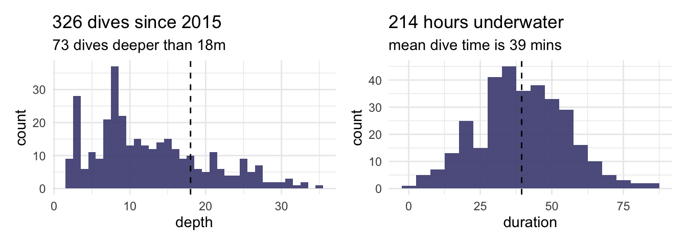

Show code

ccr_hours <- dive_log %>% 
  filter(category == "CCR") %>% 
  summarise(hrs = sum(duration) / 60) %>% 
  pull(hrs)

ccr_bar <- paste0(
  '<div style="margin: 0rem 0 0.5rem 0;">',
  '<p style="margin-bottom: 0.3rem;">',
  'I am currently working toward 50 hours on a rebreather.</p>',
  '<div style="background: #e9ecef; border-radius: 6px; ',
  'height: 32px; position: relative;">',
  '<div style="width: ', min(ccr_hours/50*100, 100), 
  '%; background: #8DA8C3; height: 100%; ',
  'border-radius: 6px;"></div>',
  '<div style="position: absolute; top: 50%; left: 10px; ',
  'transform: translateY(-50%); color: white; ',
  'font-weight: bold; font-size: 0.9rem;">',
  floor(ccr_hours), ' hours CCR</div></div></div>'
)
htmltools::HTML(ccr_bar)

I am currently working toward 50 hours on a rebreather.

14 hours CCR

Show code

map_labels <- paste0(dive_log$date, " ", dive_log$name)

dive_log %>%
  st_as_sf(coords=c('lon', 'lat')) %>% 
leaflet(options=leafletOptions(
    minZoom = 3,
    maxZoom = 10,
  )) %>% 
  setView(lng = 115, lat = -26, zoom = 4) %>% 
  addProviderTiles(provider = providers$CartoDB.Voyager) %>% 
  addCircleMarkers(radius = 7, label = map_labels,
                   stroke = FALSE, fillOpacity = .7,
                   clusterOptions = markerClusterOptions(
                     maxClusterRadius=30,
                     spiderfyDistanceMultiplier=1.2))

Show code

dive_log %>% 
  select(date, time, mins = duration,
         depth, place, category, name) %>% 
  mutate(time = substr(time,1,5)) %>% 
datatable(filter = 'top',
          class = 'compact nowrap',
          options = list(scrollX = TRUE,
                         pageLength=25,
  order = list(list(1, 'desc'),list(2, 'desc'))
))