As part of the Dating Murujuga’s Rock Art Project, I am modelling how the Ngarda-Ngarli (Traditional Custodians of Murujuga) may have voyaged throughout the archipelago in the past. The patterns of wind throughout the last several thousand years will be important to this story, and the first step is understanding what that winds are like today. The are multiple synoptic types that drive different wind components, which will require a full formal analysis later on in my project.
Climate Background
Murujuga has a hot and persistently dry desert climate (Bureau of Meteorology 2011). There is a warm/dry winter from May-November, and a hot/wet summer from December to March (Department of Environment and Conservation 2013). In winter, winds are are easterly to southerly, and in summer strong south-westerly through north-westerly (Semeniuk and Wurm 1987). Land-breezes and sea-breezes operate throughout the year, and interact with these patterns (Semeniuk and Wurm 1987).
Historical data
For this analysis we use BOM data from Legendre Island (BOM ID: 004095). This is at the north-west end of the island (-20.3583, 116.8431) at 29m altitude.
Show code
library(tidyverse)
library(lubridate)
library(leaflet)
library(viridis)
theme_set(theme_minimal())

wind_raw <- read_csv("data/HC06D_Data_004095_9999999910009138.csv")

wind <- wind_raw %>%
  mutate(date = make_datetime(
    year = as.numeric(Year),
    month = as.numeric(Month),
    day = as.numeric(Day),
    hour = as.numeric(Hour),
    min = as.numeric(`Minute in Local Standard Time`),
    tz = "Australia/Perth"
  )) %>% select(date,
                "speed" = `Wind speed measured in km/h`,
                'speed_q' = `Quality of wind speed`,
                'dir' = `Wind direction measured in degrees`,
                'dir_q' = `Quality of wind direction`) %>%
  filter(!is.na(date))

leaflet() %>%
  addProviderTiles(providers$CartoDB.Positron) %>%
  addMarkers(lng=116.8431, lat=-20.3583,
             label="Legendre Island (BOM ID: 004095)") %>%
  setView(116.8431, -20.51, zoom = 10)
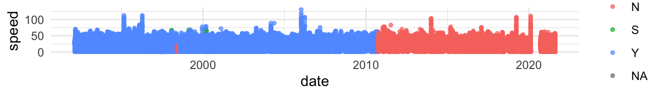
It has 217,172 observations between 1992-02-17 and 2021-08-10. Only data before October 2010 is quality controlled, but prior to that there are very few suspect measures. There are substantial gaps in 2018 and 2020. We have not filtered the data in the following analysis.
Show code
ggplot(wind) +
  geom_point(aes(date, speed, colour = speed_q), alpha=0.7, size=1)
Seasonality
General trends
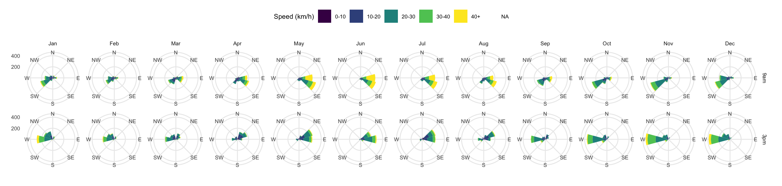
The dominant summer pattern is a west-south-westerly wind in the mornings, shifting to a westerly in the afternoon. It reverses in March to the winter pattern, with a strong east-south-easterly in the morning, and a east-north-easterly in the afternoon. Around September the summer pattern returns.
Show code
#https://stackoverflow.com/questions/17266780/wind-rose-with-ggplot-r
wind %>%
  filter(hour(date) %in% c(9,15)) %>%
  mutate(bin = cut(speed,
                   breaks=c(0, 10, 20, 30, 40, Inf),
                   labels=c("0-10","10-20","20-30", '30-40', '40+')),
         hour = case_when(
           hour(date) == 9 ~ '9am',
           hour(date) == 15 ~ '3pm'
         )) %>%
  ggplot(aes(dir)) + geom_histogram(aes(fill=bin), binwidth=30,
                                    position = position_stack(reverse = TRUE)) +
  coord_polar(start = -22.5/2*pi/180) +
  scale_x_continuous(name = "", limits = c(0 - 22.5/2, 360 - 22.5/2),
                       breaks = seq(0, 360 - 45, by = 45),
                       minor_breaks = NULL,
                       labels = c("N", "NE", "E", "SE",
                                  "S", "SW", "W", "NW")) +
  labs(fill="Speed (km/h)", y=NULL) +
  scale_y_continuous(breaks = c(200,400)) +
  facet_grid(cols = vars(month(date, label=TRUE)),
             rows = vars(fct_relevel(hour,'9am','3pm'))) +
  scale_fill_viridis(discrete=TRUE) +
  theme(legend.position="top", text = element_text(size=8)) +
  guides(fill = guide_legend(nrow = 1))
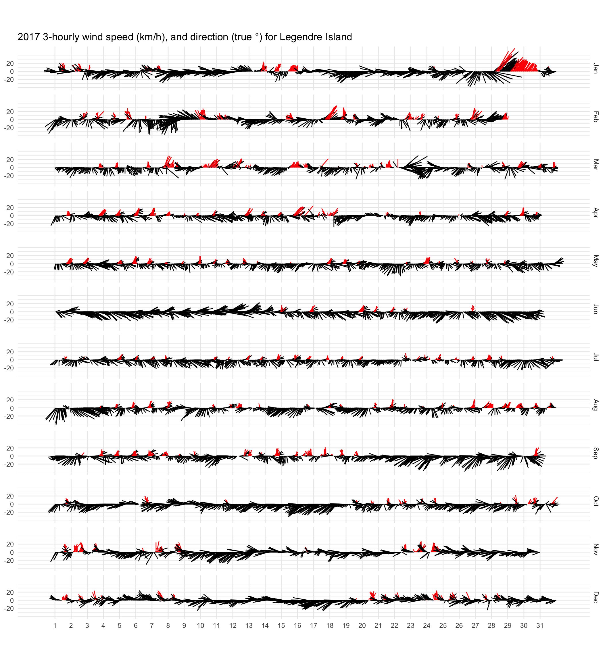
2017 example
The last set of continuous yearly data is from 2017. In the graph below, line length is proportional to wind strength, and direction points towards wind origin. The daily pattern is relatively consistent, with instability during transition periods in March and September. Choosing representative days, it is possible to see the synoptic patterns driving this weather.
The summer westerlies are associated with the Australian monsoon. This establishes cyclonic flow, with low-pressure over the north west of the continent pulling in moist ocean air. During the day, the pressure over the continent drops, strengthening the flow. Murujuga is positioned at the top of this system when it is at its strongest, so the southerly component disappears. See November the 10 to 15th 2017 for an example.
In the winter, the northerly afternoon component is driven by wind coming down the coast. As the continent heats up during the day, it appears to form an area of low pressure along the coast, which air flows along. It seems to be quite a specific regional effect, driven by the shape of the coastline. See June 8th 2017 for an example.
I have also highlighted the northerly winds. These are interesting because sustained northerlies are not a major feature of the current climate, but large paleo-dunes suggest they were in the past. As part of my project, there will be more work to understand what drives those, and what they suggest about the broader climate state.
Show code
year <- 2017
tidywind <- wind %>%
  filter(year(date) == year) %>%
  mutate(day = day(date),
         mhour = (day-1)*24 + hour(date),
         month = month(date, label = TRUE),
         speed = speed)

c <- 3/5 #controls aspect ratio

#Inspired by: https://www.py4u.net/discuss/875769

ggplot(tidywind) +
  geom_segment(aes(x = mhour,
                   y = 0,
                   xend = mhour - c*(
                     speed * 1 * -cos((90-dir) / 360 * 2 * pi)),
                   yend = (speed * sin((90-dir) / 360 * 2 * pi)),
                   colour = (dir<45|dir>325),
  )) +
  coord_fixed(c) +
  scale_x_continuous(breaks = (0:30)*24-1,
                     labels = 1:31, minor_breaks = NULL) +
  facet_grid(row = vars(month)) + labs(x=NULL, y=NULL,
         title = "2017 3-hourly wind speed (km/h), and direction (true °) for Legendre Island") +
  scale_y_continuous(breaks = c(-20,0,20)) +
  scale_colour_manual(values=c('black', 'red')) +
  theme(legend.position = "none")